Pricing vs Valuation

import numpy as np
import matplotlib.pyplot as plt
import scipy as sp
import pandas as pd

plt.style.use("ggplot")

In general, derivative pricing follows the no-arbitrage rule. In other words, the price of a derivative should equal the discounted future cash flow.

Pricing refers to the price of underlying assets (no-arbitrage principle), while valuation pertains to the pricing of contracts (risk neutrality).

Risk neutrality is a vital assumption because there are three types of investors in the market: risk-averse, risk-prone, and risk-neutral investors. Each type of investor will have their own view of future asset prices and, therefore, a different discount rate. However, this could lead to different prices in financial markets, which would be arbitraged away immediately. Consequently, all investors converge their valuation approaches based on risk neutrality.

Risk-neutral investors do not expect a risk premium, which guarantees that the pay-off can be discounted by the risk-free rate.

Options

Call Options

Call option is the right to buy a particular asset for an agree price \(E\) at time \(T\) in the future.

For instance, you bought a call option to buy a share of Lululemon in \(T=3\) months (expiry) at price of \(K=\$350\) (strike price). If today Lululemon’s price is \(P=\$200\), i.e. \(P<K\), is the called out of money, \(P=K\) at the money and \(P>K\) in the money.

At the expiry, the option’s price is obvious, only two possibilities \[ \max{(S-K, 0)} \] that means equals either asset price minus strike price, or zero.

Put Options

Put option is the right to sell a particular asset for an agree price \(E\) at time \(T\) in the future.

For instance, you bought a put option to sell a share of Lululemon in \(T=3\) months (expiry) at price of \(K=\$200\) (strike price). Today Lululemon’s price is \(\$350\).

At the expiry, the option’s price has only two possibilities \[ \max{(E-K, 0)} \] that means equals either strike price minus asset price, or zero.

American vs European Options

The American options can be exercised at any \(t<T\) time before expiry, in contrast the European options can only be exercised at \(T\) time on expiry.

Some literature differentiate continuous and discrete process by denoting \(X(t)\) or \(X_t\), we will not differentiate the notation, unless it’s necessary.

Wiener Processes and GBM

Using mathematical jargon, a stochastic process is defined on a probability space \((\Omega, F, P)\), where \(\Omega\) is a nonempty sample space, \(F\) is a \(\sigma\)-algebra (the power set of all possible subsets of \(\Omega\)), and \(P\) is a probability measure.

The Wiener process is a stochastic process denoted as \(W_t\). The process is defined as: \[ \Delta W_t = W_{t+\Delta t} - W_t = \epsilon \sqrt{\Delta t};\\ W_t = O(\sqrt{\Delta t}) \] \[ W_{t+\Delta t} - W_t \sim N(0, \Delta t) \]

where \(O\) is the big-O nation for order. A geometric random walk model is defined as: \[ \Delta S = \mu S \Delta t + \sigma S \Delta W = \mu S \Delta t + \sigma S \epsilon \sqrt{\Delta t} \] where:

• \(\Delta S\): change in stock price, \(S_{t+\Delta t}\)
• \(\mu S \Delta t\): \(\mu\) is the expected return rate, representing the deterministic trend
• \(\sigma S \Delta W\): \(\sigma\) is the standard deviation of the stock, and \(\epsilon\) follows a standard normal distribution

This is the fundamental model for derivative pricing.

def wiener_process(dt=0.1, x0=0, n=1000):
    W = np.zeros(n + 1)
    t = np.linspace(x0, n, n + 1)
    W[1 : n + 1] = np.cumsum(np.random.normal(0, np.sqrt(dt), n))
    return t, W


def plot_process(t, w):
    fig, ax = plt.subplots(figsize=(12, 6))
    ax.plot(t, W)
    ax.set_xlabel("Time")
    ax.set_ylabel("Wiener Process")
    plt.show


if __name__ == "__main__":
    t, W = wiener_process()
    plot_process(t, W)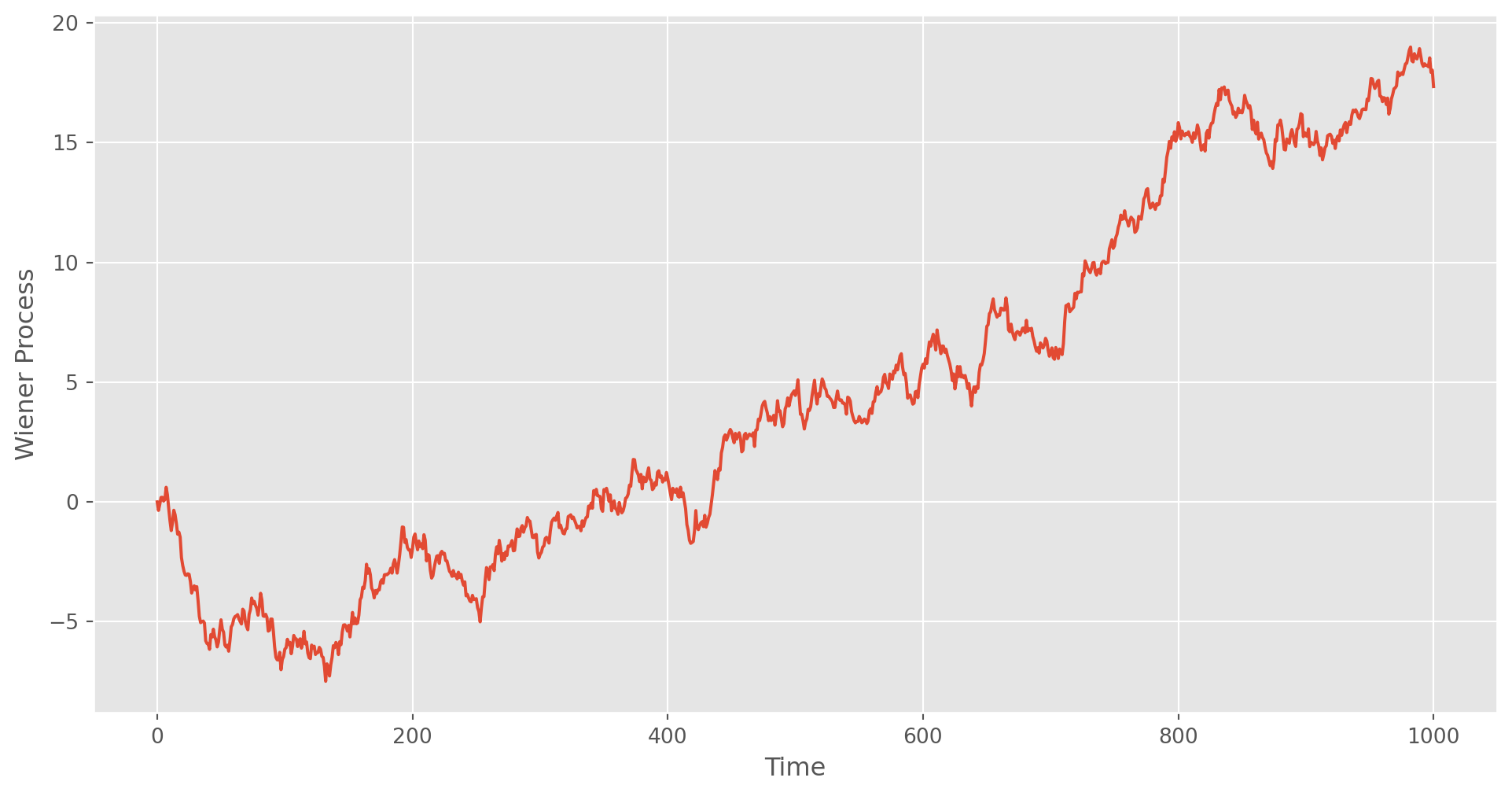

The Brownian motion , sometimes also know as Standard Wiener Process, is a fractal in nature, the function will not be differentiable with a well-defined gradient. A standard Brownian motion has following characteristics

\[ \begin{aligned} W(0) & =0 \text { a.s. } \\ E[W(t)] & =0(\mu=0) \\ E\left[W^2(t)\right] & =t\left(\sigma^2=1\right) \end{aligned} \]

However, due to fractal nature \[ \frac{W_t}{t} \] does not exist.

Itô Processes

An Itô process is a generalized Wiener process, \(n\)-dimensional representation is \[ S_t=S_0+\int_0^t a(S_s,s) d s+\int_0^t b(S_s, s) d W_s \]

where \(a\) and \(b\) can be \(n\)-dimensional variable or constants, the former models the asset growth rate , the latter models the magnitude of volatility, \(W_s\) a standard Brownian motion process. \(X_t\) is the current stock price, \(X_0\) the initial stock price.

The first integral adds up growth in every period, i.e. accumulative growth \[ E(S_t) = \int_0^t a_s d s \]

The second integral adds up all volatilities from Wiener process.

\[ \text{Var}{(S_t)} = \int_0^t b_s d W_s \]

The differential version of Itô Process is $$ d S_t=a(S_t, t) d t+b(S_t, t) d W_t

where \(a(X_t, t)\) and \(b(X_t, t)\) are deterministic functions of growth rate and volatility of stochastic process \(S_t\) and \(t\).

Compare with the GBM we have derived in Chapter 0, the Itô process is a more general form of stochastic process. \[ d S=\mu S d t+\sigma S d W \] that in Ito process \(a=\mu S\) and \(b=\sigma S\).

Itô’s Lemma

Itô’s Lemma is a stochastic version of the Taylor expansion, it is used to find the differential of a function of a stochastic process. Now imagine a price of an otpion is defined as a function of stock price and time \[ V(S, t) \]

Let’s do a standard Taylor expansion to second order on \(\Delta V = V(S+\Delta S, t+\Delta t)-V(S, t)\) \[ \begin{aligned} \Delta V & =V(S+\Delta S, t+\Delta t)-V(S, t) \\ & =\frac{\partial V}{\partial S} \Delta S+\frac{\partial V}{\partial t} \Delta t+\frac{1}{2} \frac{\partial^{2} V}{\partial S^{2}}(\Delta S)^{2}+\frac{1}{2} \frac{\partial^{2} V}{\partial t^{2}}(\Delta t)^{2}+\frac{\partial^{2} V}{\partial S \partial t} \Delta S \Delta t \tag{2} \end{aligned} \]

The discrete form of Itô’s Lemma is \[ \begin{aligned} \Delta S = \mu \Delta t + \sigma \epsilon \sqrt{\Delta t} \\ \end{aligned} \] And take square of both sides \[ \begin{aligned} (\Delta S)^2 & = \mu^2(\Delta t)^2+\sigma^2 \epsilon^2 \Delta t+2 \mu \sigma \epsilon(\Delta t)^{3 / 2}=\sigma^2 \epsilon^2 \Delta t+H(\Delta t) \end{aligned} \] \(H\) denotes higher order terms. But this tells that \((\Delta S) ^2 = O(\Delta t)\), we can’t drop $(S) ^2 $ due to the same reason we don’t drop \(\Delta t\).

Recall that we have mentioned in Chapter 0 that as \(\Delta t \rightarrow 0\), that \(\Delta S\) will be dominated by \(\sigma \epsilon \sqrt{\Delta t}\), i.e. \((\Delta S)^2 = \sigma^2d t\).

Combine the above results setting \(\Delta t \rightarrow 0\), the equation \((1)\) becomes a differential form \[ \begin{aligned} d V =\frac{\partial V}{\partial S} d S+\frac{\partial V}{\partial t} d t+\frac{1}{2} \frac{\partial^{2} V}{\partial S^{2}}\sigma^2 d t \end{aligned} \]

Collecting terms and combine with \((1)\), we have the famous Itô’s Lemma $$ \[\begin{aligned} d V =\left(\frac{\partial V}{\partial t}+\mu S \frac{\partial V}{\partial S}+\frac{1}{2} \sigma^2 S^{2} \frac{\partial^{2} V}{\partial S^{2}}\right) d t+\sigma S \frac{\partial V}{\partial S} d W \tag{3} \end{aligned}\]

The Well-Known Use Case of Itô’s Lemma

Here we will demonstrate a well-known use case of Itô’s Lemma, the forward contract is priced by the following formula \[ F=S e^{r(T-t)} \] Assuming the stock price is given by \[ d S=\mu S d t+\sigma S d W \]

According to Itô’s Lemma, we prepare following derivatives \[ \begin{gathered} \frac{\partial F}{\partial S}=e^{r(T-t)}, \quad \frac{\partial^2 F}{\partial S^2}=0, \quad \frac{\partial F}{\partial t}=-r S e^{r(T-t)} \end{gathered} \]

Plug in the Itô’s Lemma \[ d F=\left(e^{r(T-t)} \mu S-r S e^{r(T-t)}+0(\sigma X)^2\right) d t+e^{r(T-t)} \sigma S d W \]

Substitute \(F=S e^{r(T-t)}\)

\[ d F=(\mu-r) F d t+\sigma F d W \]

Itô’s Lemma allows to make predictions of forward price based on stock (asset) price.

Log Example

Assume an \(F\) function takes a natural log form \[ F(S)=\log S(t) \]

Prepare derivatives \[ \begin{gathered} \frac{\partial F}{\partial S}=\frac{1}{S(t)}, \quad \frac{\partial^2 F}{\partial S^2}=-\frac{1}{S(t)^2}, \quad \frac{\partial F}{\partial t}=0 \end{gathered} \]

Plug into Itô’s Lemma

\[ d F(S)=\frac{1}{S} d S-\frac{1}{2} \frac{1}{S^2} d S^2 \]

Substitute \(S\) by geometric Brownian motion process \[ d F(S)=\frac{1}{S}(\mu S d t+\sigma S d W)-\frac{1}{2} \frac{1}{S^2} \sigma^2 S^2 d t \\ d F(S)=\left(\mu-\frac{1}{2} \sigma^2\right) d t+\sigma d W \]

Integrate \(dF(S)\) on both sides and apply natural log on \(F(S)=\log S(t)\) \[ S(t)=S(0) e^{\left(\mu-\frac{1}{2} \sigma^2\right) t+\sigma W_t} \]

So, the example means if \(F(S)\) is a derivative of \(S\), \(S(t)\) can be obtained by Itô’s Lemma.

Here’s the code to simulate the log example, note that the simulated stock will never be able to cross \(0\) line, which is a good feature for simulating assets price.

def sim_geometric_rw(S0, T=10, N=1000, mu=0.1, sigma=0.05):
    dt = T / N
    t = np.linspace(0, T, N)
    W = np.random.normal(0, 1, size=N)  # standard Wiener process
    W = np.cumsum(W) * np.sqrt(dt)  # scale the st.dev. into sqrt(t)
    F = (mu - 0.5 * sigma) * t + sigma * W
    S = S0 * np.exp(F)
    return t, S


def plot_simu(t, S):
    fig, ax = plt.subplots(figsize=(12, 6))
    ax.plot(t, S)
    ax.set_xlabel("Time")
    ax.set_ylabel("Stock Price")
    ax.set_title(r"$S(t)=S(0) e^{\left(\mu-\frac{1}{2} \sigma^2\right) t+\sigma W_t}$")
    plt.show()


if __name__ == "__main__":
    time, data = sim_geometric_rw(S0=1, T=10, N=1000, mu=0.1, sigma=0.3)
    plot_simu(time, data)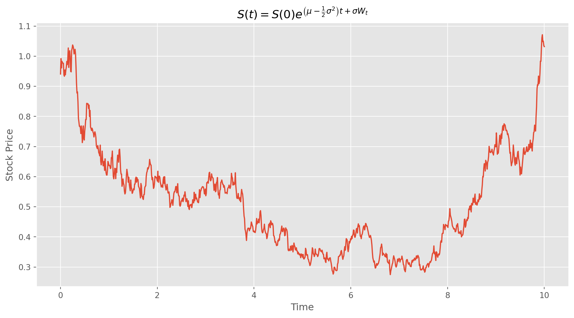

Options Pricing

Denote an option’s price as \(V(S,t)\), where \(S\) is the underlying stock price modeled by \[ d S_t=a\left(S_t, t\right) d t+b\left(S_t, t\right) d W_t \]

Give it a full Taylor expansion till \(2\)-nd order \[ {V}({S}+\Delta {S}, {t}+\Delta {t})={V}({S}, {t})+\frac{\partial {V}}{\partial {t}} \Delta {t}+\frac{\partial {V}}{\partial {S}} \Delta {S}+\frac{1}{2}\left(\underbrace{\frac{\partial^2 {~V}}{\partial {t}^2} \Delta {t}^2+2 \frac{\partial^2 {~V}}{\partial {S} \partial {t}} \Delta {S} \Delta {t}}_{\approx 0}+\frac{\partial^2 {~V}}{\partial {S}^2} \Delta {S}^2\right) \]

Rearrange the equation, i.e. moving \(V(S, t)\) to the left \[ dV( {S}, {t})=\frac{\partial {V}}{\partial {t}} {dt}+\frac{\partial {V}}{\partial {S}} {dS}+\frac{1}{2} \frac{\partial^2 {~V}}{\partial {S}^2} {dS}^2 \]

The last term \(dS^2\) is actually \((dS)^2\), but usually parentheses are omitted to avoid jamming notation, so plug in the geometric Brownian motion model into \(dS\) and omit arguments of \(a\) and \(b\) \[ d S^2=(a d t+b d W)^2=\underbrace{a^2 d t^2+2 a b d t d W}_{\approx 0}+b^2 d W^2=b^2 d W^2 \]

Recall the Wiener process definition that \[ E(dW^2) = dt \]

Therefore \[ d V(S, t)=\frac{\partial V}{\partial t} d t+\frac{\partial V}{\partial S} d S+\frac{1}{2} b^2 \frac{\partial^2 V}{\partial S^{2}} d t \]

Black-Scholes Model

Black and Scholes (1973) shows that even systematic risk can be eliminated by including risky assets, which generates market-neutral strategy such as delta-hedging and pairs-trading.

In a full-fledged option’s price function, there are following parameters \[ V(S, t, \sigma, \mu, K, T, r) \] \(S\): stock price, following an Itô process \(d S=\mu S d t+\sigma S d W\)
$ \(t\): time
\(\sigma\): volatility
\(\mu\): mean of stock price growth
\(K\): strike price
\(T\): expiry
\(r\): risk-free rate

We can construct a portfolio which eliminate risk at this moment \(t\), i.e. long a contract of call option and short \(\Delta\) quantity of underlier \(S\). \[ \Pi = V(S, t) - \Delta S \] Because there are some level of correlation between stock price and options pay-off, with this portfolio we can eliminate all risks.

Now suppose time elapsed a bit, all variables have a marginal change too. \[ d \Pi = dV(S, t) - \Delta dS \] where \(\Delta\) is assumed to be constant for the time being, this is unrealistic, but simplifies our deduction process.

Plug into portfolio’s equation with \(dS = \mu S dt + \sigma S dW\) and \(dV\) from Itô’s Lemma \[ \begin{aligned} {d} \Pi&=\underbrace{\left(\frac{\partial V}{\partial t}+\mu S \frac{\partial V}{\partial S}+\frac{1}{2} \sigma^2 S^2 \frac{\partial^2 V}{\partial S^2}\right) d t+\sigma S \frac{\partial V}{\partial S} d W}_{\text{Itô's Lemma}}-\underbrace{\Delta\left(\mu S d t+\sigma S d W\right)}_{dS}\\ &=\left(\frac{\partial V}{\partial t}+\mu S \frac{\partial V}{\partial S}+\frac{1}{2} \sigma^2 S^2 \frac{\partial^2 V}{\partial S^2}-\Delta \mu S\right) d t+\left(\sigma S \frac{\partial V}{\partial S}-\Delta \sigma S\right) d W\\ &=\left(\frac{\partial V}{\partial t}+\underbrace{\mu S \frac{\partial V}{\partial S}-\Delta \mu S}_{=0} +\frac{1}{2} \sigma^2 S^2 \frac{\partial^2 V}{\partial S^2} S\right) d t+\left(\sigma S \frac{\partial V}{\partial S}-\Delta \sigma S\right) d W\\ &=\underbrace{\left(\frac{\partial V}{\partial t}+\frac{1}{2} \sigma^2 S^2 \frac{\partial^2 V}{\partial S^2}\right) d t}_{\text{deterministic}}+\underbrace{\left(\sigma S \frac{\partial V}{\partial S}-\Delta \sigma S\right) d W}_{\text{stochastic}} \end{aligned} \] any terms with \(dt\) are deterministic (drift) and terms with \(dW\) are stochastic (diffusion).

But why are we doing this?

The goal is to construct a portfolio which eliminates risks, what does it mean in terms of \(d\Pi\)?

If no risks, then \(d\Pi\) should be a constant, since it contains both a deterministic and stochastic term, eliminating risks means to force stochastic terms equal to \(0\)!

That means \[ \frac{\partial V}{\partial S} - \Delta = 0 \] which is exactly the mathematical definition of the Greek \(\Delta\).

Black-Scholes PDE

The Delta-hedging strategy aims to achieve \[ \frac{\partial V}{\partial S}=\Delta \] which renders the stochastic part \(0\).

To maintain this hedging position, \(\Delta\) has to be dynamically balanced. Once this condition is achieved, there is only riskless part in the portfolio, and portfolio became fixed income asset \[ d\Pi = r \Pi dt \] where \(r\) is risk-free rate.

So we end up having two portfolios, one involves options and underlying assets, one is a riskless fixed income. They both are riskless and should have the same \(d\Pi\).

Use the deterministic part of \(d\Pi\) and \(\Pi=V(S, t) - \Delta S\), also assuming \(\frac{\partial V}{\partial S}=\Delta\)

\[ d\Pi = \left(\frac{\partial {V}}{\partial {t}}+\frac{{1}}{{2}} \sigma^2 S^2 \frac{\partial^2 {V}}{\partial S^2}\right) {d t}={r}\left({V}-{S} \frac{\partial {V}}{\partial {S}}\right) {d t} \]

Arrange the equation, we get the famous Black-Scholes equation

\[ \begin{gathered} \underbrace{\frac{\partial V}{\partial t}}_{\Theta}+\frac{1}{2} \sigma^2 S^2 \underbrace{\frac{\partial^2 V}{\partial S^2}}_{\Gamma}+r S \underbrace{\frac{\partial V}{\partial S}}_{\Delta}-r V=0 \tag{4} \end{gathered} \]

which is a parabolic partial differential equation.

In a complete market, \(V= \Pi + \Delta S\), an option can be replicated by holding cash and \(\Delta\) shares of stocks, which makes options redundant! In other words, in order to price options, we come to a conclusion that options are unneeded, because we can always replicated it if we know \(\Delta\) at every moment.

Dividends and FX Interest Rate

The Greeks

We have seen Delta from above, \[ \Delta = \frac{\partial V}{\partial S} \] which measures the sensitivity of option.

Gamma is the derivative of \(\Delta\) \[ \Gamma = \frac{\partial^2 V}{\partial S^2} \] which measures how often a position must be re-hedged in order to maintain a delta-neutral position.

Theta is the rate of change of option over time \[ \Theta = \frac{V}{t} \]

Vega measures the sensitivity of option over stock’s volatility \[ \mathcal{V}=\frac{\partial V}{\partial \sigma} \] However note that \(\mathcal{V}\) is not real Greek letter, it is simply a larger size \(\nu\) (nu).

With these Greeks, we can rewrite Black-Scholes as \[ \begin{gathered} \Theta+\frac{1}{2} \sigma^2 S^2 \Gamma+r S \Delta -r V=0 \end{gathered} \]

Implementation

We will use solution of Black-Scholes to evaluate European vanilla options

\[ \begin{align} \text{Call: }&S(0) \Phi\left(d_1\right)-E e^{-r(T-t)} \Phi\left(d_2\right) \\ \text{Put: }&-S(0) \Phi\left(-d_1\right)+E e^{-r(T-t)} \Phi\left(-d_2\right) \\ \end{align} \]

def call_option_price(S, K, T, risk_free, sigma):
    d1 = (np.log(S / K) + (risk_free + (sigma**2) / 2) * T) / (sigma * np.sqrt(T))
    d2 = d1 - sigma * np.sqrt(T)
    return S * sp.stats.norm.cdf(d1) - K * np.exp(-risk_free * T) * sp.stats.norm.cdf(
        d2
    )


def put_option_price(S, K, T, risk_free, sigma):
    d1 = (np.log(S / K) + (risk_free + (sigma**2) / 2) * T) / (sigma * np.sqrt(T))
    d2 = d1 - sigma * np.sqrt(T)
    return -S * sp.stats.norm.cdf(-d1) + K * np.exp(-risk_free * T) * sp.stats.norm.cdf(
        -d2
    )


if __name__ == "__main__":
    S0 = 95
    K = 100
    T = 0.5
    risk_free = 0.05
    sigma = 0.2
    print("Call option price: {}".format(call_option_price(S0, K, T, risk_free, sigma)))
    print("Put option price: {}".format(put_option_price(S0, K, T, risk_free, sigma)))

Call option price: 4.254540648120496
Put option price: 6.78553185095376

MCMC for Stock Simulation

First, we simulate stock price with the formula below \[ S(t)=S(0) e^{\left(\mu-\frac{1}{2} \sigma^2\right) t+\sigma W_t} \]

num_of_simu = 500


def stock_monte_carlo(S0, mu, sigma, N=252):  # 252 trading days a year
    results = []
    for i in range(num_of_simu):
        prices = [S0]
        for j in range(N):
            # simulate day by day, so no t in function
            stock_price = prices[-1] * np.exp(
                (mu - (sigma**2) / 2) + sigma * np.random.normal()
            )
            prices.append(stock_price)
        results.append(prices)
    simu_data = pd.DataFrame(results)
    simu_data = simu_data.T
    simu_data["mean"] = simu_data.mean(axis=1)
    print("Prediction for 1 year later: {}".format(simu_data["mean"].tail(1)))
    fig, ax = plt.subplots(figsize=(12, 6))
    ax.plot(simu_data)
    ax.plot(simu_data["mean"], lw=3, color="k")
    plt.show()


if __name__ == "__main__":
    stock_monte_carlo(S0=50, mu=0.0003, sigma=0.01)

Prediction for 1 year later: 252    53.373962
Name: mean, dtype: float64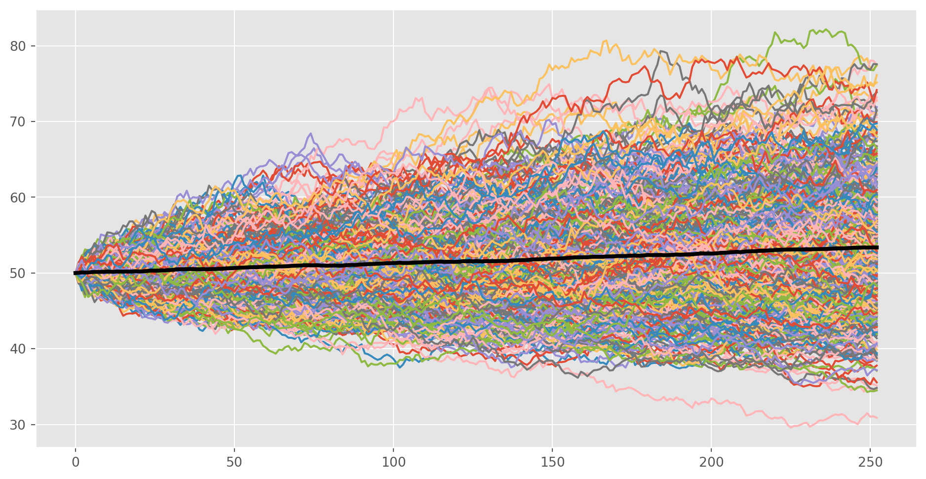

MCMC for Options Pricing

If we assume risk-neutrality, we can use risk-free rate \(r\) to replace \(\mu\) \[ S(t)=S(0) e^{\left(r-\frac{1}{2} \sigma^2\right) t+\sigma \sqrt{t}N(0,1)} \]

class OptionPricing:
    def __init__(self, S0, K, T, rf, sigma, iterations):
        self.S0 = S0
        self.K = K
        self.T = T
        self.rf = rf
        self.sigma = sigma
        self.iterations = iterations

    def call_option_simu(self):
        # placeholder for max(0, S-K)
        option_data = np.zeros([self.iterations, 2])
        W = np.random.normal(0, 1, [1, self.iterations])  # wienar process
        stock_price = self.S0 * np.exp(
            (self.rf - 0.5 * self.sigma**2) * self.T + self.sigma * np.sqrt(self.T) * W
        )
        option_data[:, 1] = stock_price - self.K
        average = np.sum(np.amax(option_data, axis=1)) / self.iterations
        return np.exp(-self.rf * self.T) * average

    def put_option_simu(self):
        # placeholder for max(0, K-S)
        option_data = np.zeros([self.iterations, 2])
        W = np.random.normal(0, 1, [1, self.iterations])  # wienar process
        stock_price = self.S0 * np.exp(
            (self.rf - 0.5 * self.sigma**2) * self.T + self.sigma * np.sqrt(self.T) * W
        )
        option_data[:, 1] = self.K - stock_price
        average = np.sum(np.amax(option_data, axis=1)) / self.iterations
        return np.exp(-self.rf * self.T) * average


if __name__ == "__main__":
    model = OptionPricing(S0=100, K=110, T=0.5, rf=0.03, sigma=0.2, iterations=1000)
    print("Value of call option: {:.2f}.".format(model.call_option_simu()))
    print("Value of put option: {:.2f}.".format(model.put_option_simu()))

Value of call option: 2.13.
Value of put option: 11.11.